
Inbound lead scoring to optimize marketing spend is a very common starting project for a new data science team. As a b2b business matures, it accrues a significant number of daily visitors to its website that sign up to talk to a salesperson, learn more about the product, or try a free trial. Some of these visitors (“leads” in sales parlance) are promising future customers. But many are just kicking the tires. Separating the wheat from the chaff is a classic data science problem.
In this post we’ll take a pretty classic lead scorer and show how it can be deployed to two places:
- A REST endpoint, where it can be called from your website.
- A data warehouse, where it can make predictions in batch, and also have those predictions reverse ETL’d into our CRM.
Getting the training data into shape
We’ll start by building a somewhat realistic lead scorer: An SKLearn Pipeline containing an XGBoost regressor. We chose them simply because they’re very common choices for lead scoring models. The purpose of the regressor is to provide a probability of a binary outcome: How likely is the lead to convert into a paying customer?
We’ll start with a DataFrame that has the three features we’ll use in our model: the source of the lead, the size of the company, and the industry it’s in. We’ve also got the ground truth of whether they converted or not in the “converted_to_customer” column.
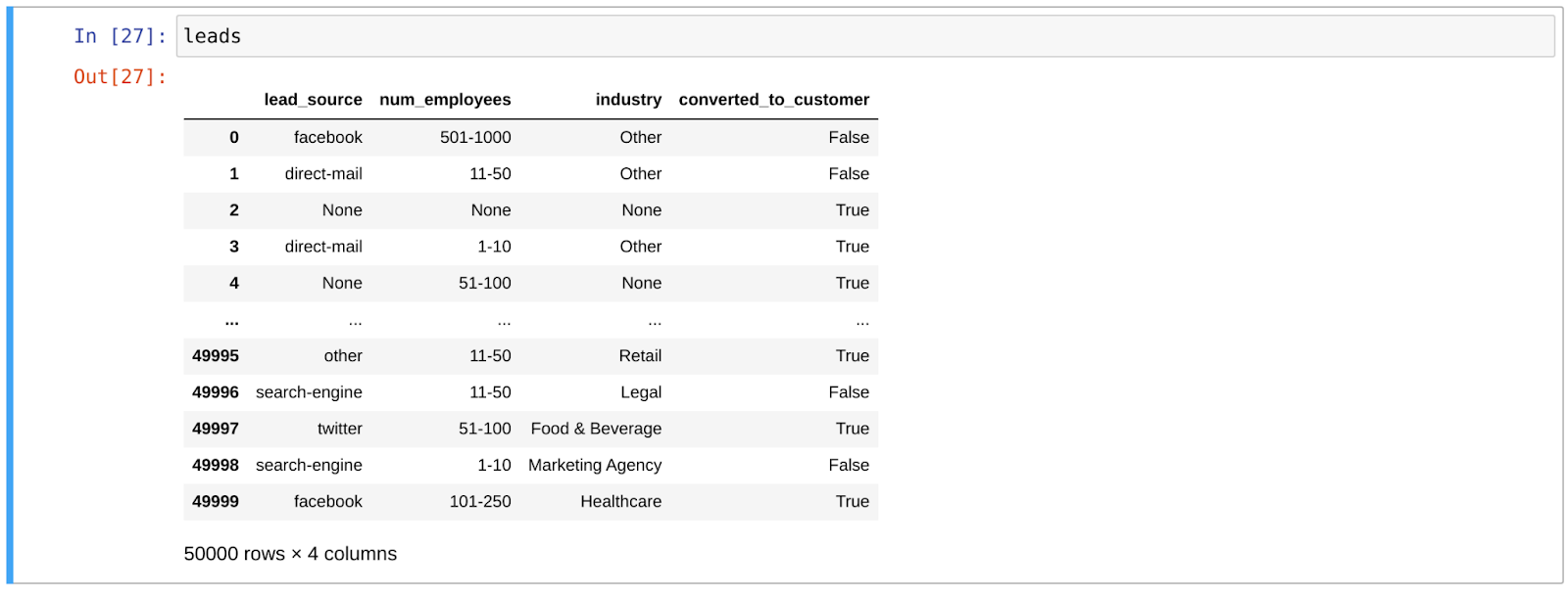
In total, a training set of 50,000 leads to work with.
Our “lead_source” and “industry” columns are simple category features. We’ll leave them as-is when building our training DataFrame, and encode them inside the model pipeline later on:
{%CODE python%}
X = leads[["lead_source", "industry"]]
{%/CODE%}
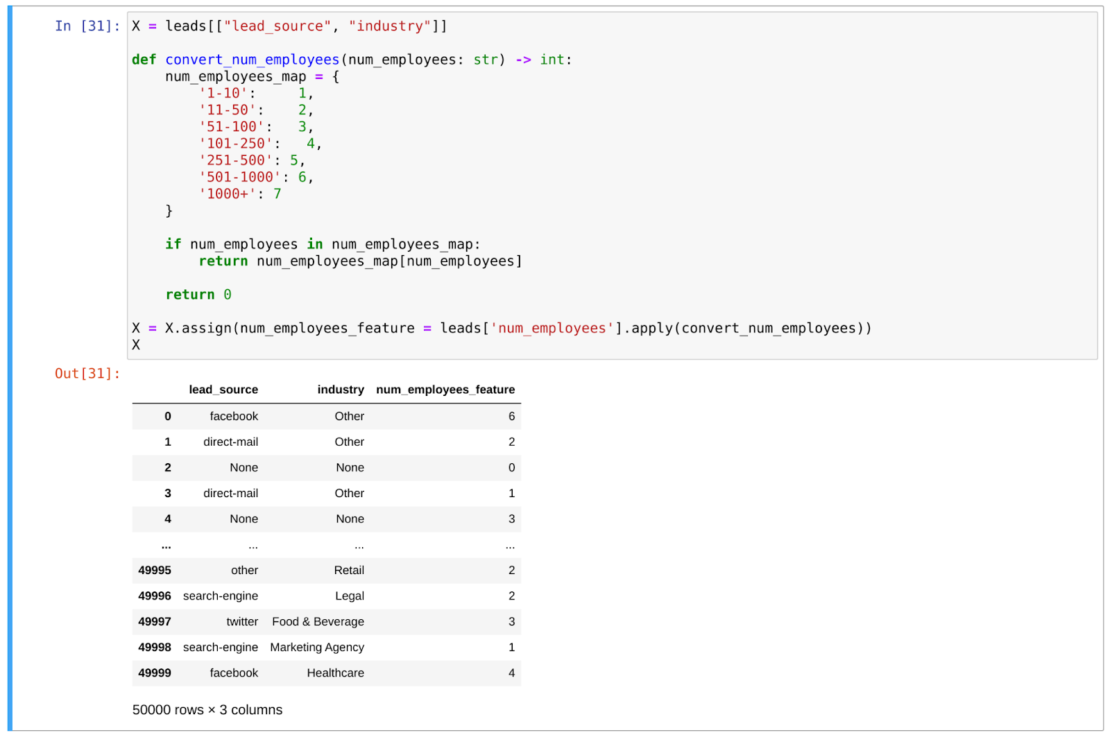
The “num_employees” column is more interesting though. While the data type is string, the values represent numeric ranges, and we definitely want the model to understand that “11-50” employees is more than “1-10” employees and so on. So let’s engage in a little custom feature engineering:
{%CODE python%}
def convert_num_employees(num_employees: str) -> int:
num_employees_map = {
'1-10': 1,
'11-50': 2,
'51-100': 3,
'101-250': 4,
'251-500': 5,
'501-1000': 6,
'1000+': 7
}
if num_employees in num_employees_map:
return num_employees_map[num_employees]
return 0
{%/CODE%}
With this function, we transform our “num_employees” column into a “num_employees_feature” that’s a value from 0 to 7.
Putting it all together, we’ve got our training DataFrame.
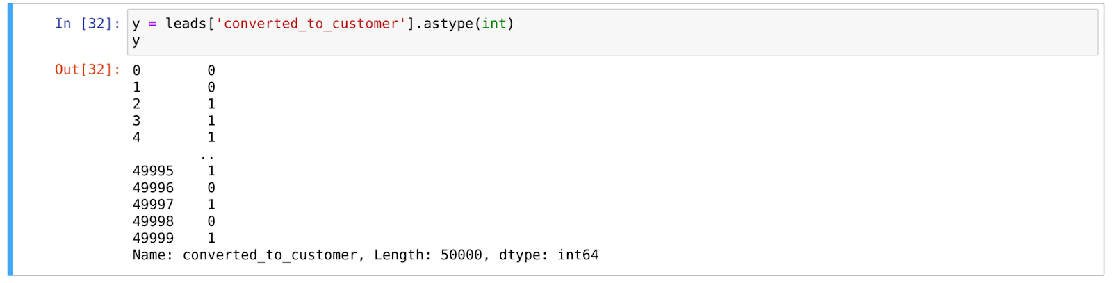
Finally, we need to transform our boolean “converted_to_customer” target column to a number so that the regression can understand it:
Fitting the model
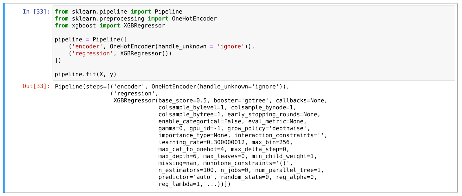
Alright, let’s fit the model! As I mentioned, many of the models we see are XGBoost regressors, so let’s start there. And because we have a couple category features, let’s drop it in an SKLearn pipeline with a OneHotEncoder. All together, it looks pretty simple:
{%CODE python%}
from sklearn.pipeline import Pipeline
from sklearn.preprocessing import OneHotEncoder
from xgboost import XGBRegressor
pipeline = Pipeline([
('encoder', OneHotEncoder(handle_unknown='ignore')),
('regression', XGBRegressor())
])
pipeline.fit(X, y)
{%/CODE%}
XGBRegressor is a wrapper provided by the XGBoost library that implements the Scikit-Learn API so it can be dropped right into a Scikit-Learn Pipeline, as we’ve done here. Here it is with the outputs:
At this point, we would ideally have split our data for training and testing, and would score the model in a domain-appropriate way. But we’ll skip over those steps as the purpose of this post is the deployment.
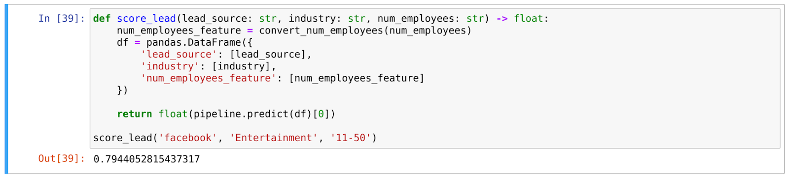
To start, let’s write a function that will call our model with the data we’ll get in production: the original lead_source, num_employees and industry values:
{%CODE python%}
def score_lead(lead_source: str, industry: str, num_employees: str) -> float:
num_employees_feature = convert_num_employees(num_employees)
df = pandas.DataFrame({
'lead_source': [lead_source],
'industry': [industry],
'num_employees_feature': [num_employees_feature]
})
return float(pipeline.predict(df)[0])
score_lead('podcast', 'Entertainment', '11-50')
{%/CODE%}
Notice we're relying on some code we wrote early. The "convert_num_employees" function is the same one we wrote when we were creating that feature. And, of couse, "pipeline" is our Scikit-Learn pipeline, which includesour One-Hot Encoder and trained XGBoost model. We're using all that code here in this function.
We can test it out locally:
Deploying to production
Now that it seems to be working, let’s deploy it! As always, we pass the function that will be called in production as an argument to Modelbit’s deploy function:
{%CODE python%}
mb.deploy(score_lead)
{%/CODE%}
Here it is in action:
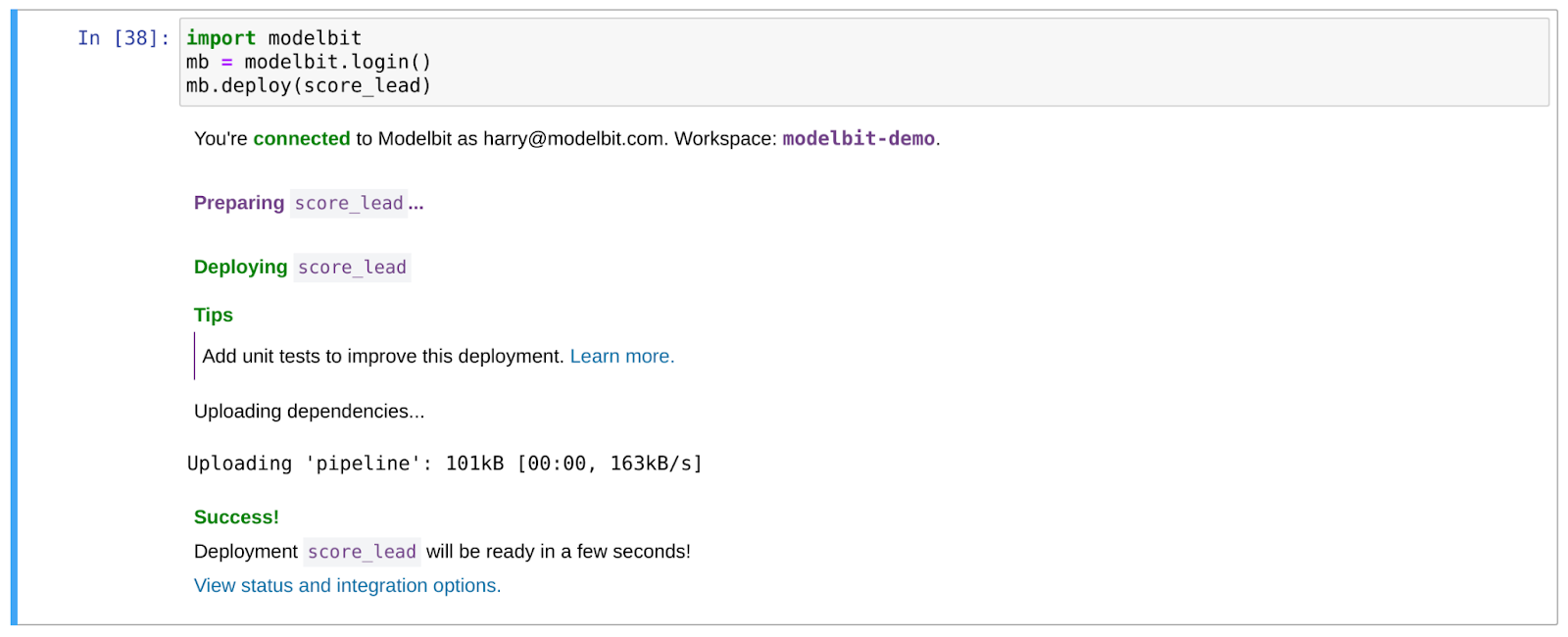
Settle down about the tests, Modelbit. 😉 I promise to add some next time!
So Modelbit is doing a number of things here. First, it’s capturing the code of the “score_lead’ function itself. It’s also capturing the data structures (i.e. “pipeline,” our Scikit-Learn pipeline) and code (i.e. the “convert_num_employees” function) that “score_lead” depends on. It will walk that dependency tree and capture all the code that runs when “score_lead” runs.
It also introspects the Python environment itself to determine what Python version and Python packages are required in production. Here that’ll be certain versions of Pandas, XGBoost and Scikit-Learn, as well as Python 3.10. But this tends to vary widely between data scientists even within a data science team.
All that is shipped to a Docker container running in a cloud environment. If we click the Modelbit link, we can see it:

Sure enough, Python 3.10, Scikit-Learn 1.0.2, Pandas 1.5.0, and XGBoost 1.6.2 are all in our production runtime. And we can see the code right there, we can rollback to old versions, and more.
Working with our model in production
But we want to actually call the model! We can see how to do that from the APIs tab:
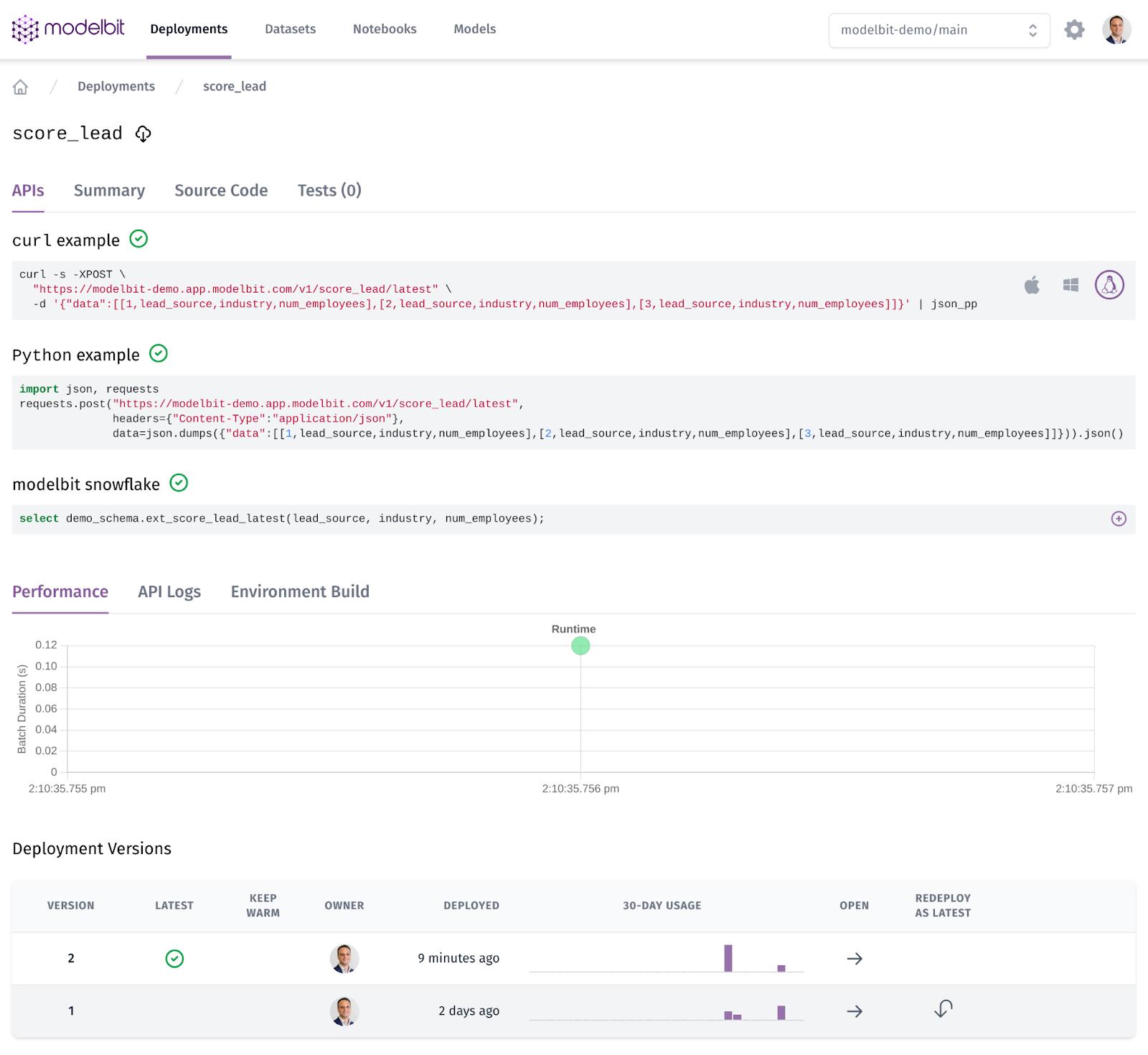
As you can see, we’ve got example code for calling it from curl, from Python and from Snowflake. The curl and Python examples hit our REST API, which lives at: https://modelbit-demo.app.modelbit.com/v1/score_lead/latest. (Go ahead, try calling it now!)
Meanwhile, the Snowflake example calls a SQL function that was automatically created in the warehouse.
We can try calling it with curl at the command line like so:
{%CODE bash%}
$ curl -s -XPOST \
"https://modelbit-demo.app.modelbit.com/v1/score_lead/latest" \
-d '{"data":[[1,"facebook", "Entertainment", "11-50"]]}' | json_pp
{
"data" : [
[
1,
0.794405281543732
]
]
}
{%/CODE%}
We get the same score from our API that we got a moment ago in the notebook!
Meanwhile we can call exactly the same code from Snowflake as well:
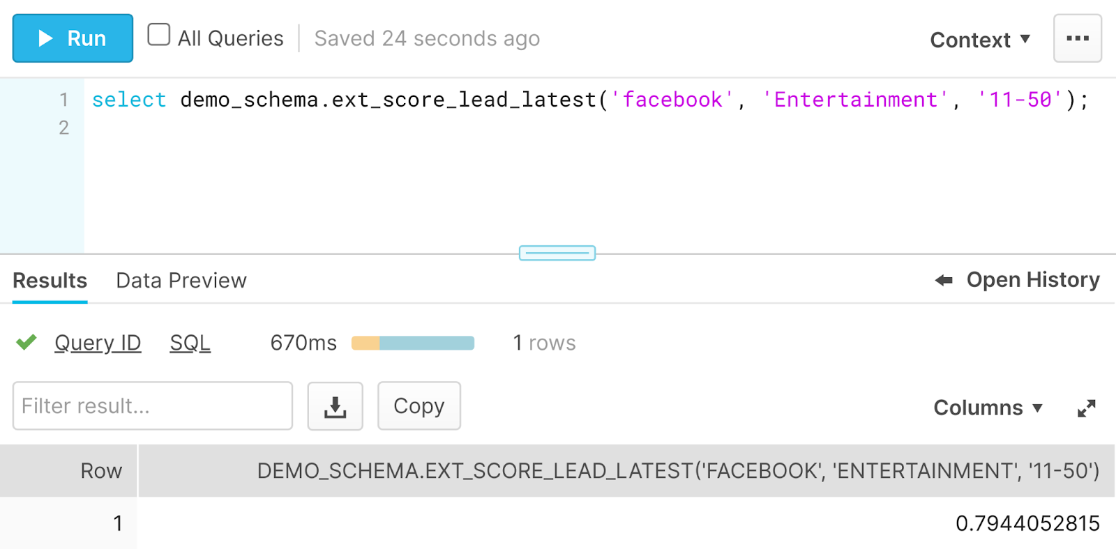
Once again, the very same prediction! Modelbit supports Redshift and other data warehouses as well, should that be your system of choice.
Here’s why this is interesting: In production, the lead scorer can be used to make realtime decisions. For example, routing a high-probability lead directly to a salesperson, whereas a low-probability lead can go to a self-signup experience. Or we can assign the lead to different salespeople depending on likelihood of conversion. Some companies use lower-quality leads as training for new salespeople, for example.
Simultaneously, the very same model can be used to write the predictions in batch in the warehouse. We could re-score all the leads and compare the new scores. Or assign scores to new leads every hour, and then reverse ETL them into our CRM with a tool like Census or Hightouch.
These two endpoints – REST API and SQL function – call exactly the same running code, enabling us to keep the model consistent even as we run it multiple places!
Definitely check it out, and download this notebook to walk through the code. In future posts, we’ll show you how to run tests, how to version control your model in git, and how to use Merge Requests or Pull Requests to deploy. Happy machine learning!
